Background
Radio signals use multiple types of modulation for encoding data (voice, music, etc.) on a carrier wave. FM – frequency modulation – is one such scheme. These signals can be analyzed by a neural network. They are essential 2d data, like an image, so CNN’s, which are great for image classification, can be used. The raw RF data is called IQ data and that stands for In-Phase and Quadrature. These are vectors containing complex numbers that represent the signal. Various RF equipment (such as a rtl-sdr USB dongle) can capture and record the data to your hard drive. GNU Radio software can also generate data for analysis, as was done by DeepSig for the work shown below that I updated.
Software Updates
I have taken a Jupyter Notebook page written for Python 2.7 and some old machine learning libraries (keras 1, for example) and updated everything so that it runs with Python 3 (3.6.8, to be precise), keras 2, and theano 1.04. To get to some of these software versions you will need to use conda-forge rather than the default conda update sites. That said, if you are here, you should know how to do this.
Throughout the original notebook I have added additional comments about what is going on to help explain the code better.
A pretty useful tool for viewing the architecture of a neural network is https://github.com/lutzroeder/netron. I highly suggest you get it.
Going from a notebook to a blog post is not a pretty process but you should just be able to take this code and add to your own Jupyter Notebook. See. https://jupyter.org/
You can find the original page here: https://github.com/radioML/examples/blob/master/modulation_recognition/RML2016.10a_VTCNN2_example.ipynb
License requirements
This work is copyright DeepSig Inc. 2017. It is provided open source under the Create Commons Attribution-NonCommercial 4.0 International (CC BY-NC 4.0) License https://creativecommons.org/licenses/by-nc/4.0/
Use of this work, or derivatives inspired by this work is permitted for non-commercial usage only and with explicit citation of this original work.
A more detailed description of this work can be found at
https://arxiv.org/abs/1602.04105
A more detailed description of the RML2016.10a dataset can be found at
http://pubs.gnuradio.org/index.php/grcon/article/view/11
Citation of this work is required in derivative works:
@article{convnetmodrec,
  title={Convolutional Radio Modulation Recognition Networks},
  author={O'Shea, Timothy J and Corgan, Johnathan and Clancy, T. Charles},
  journal={arXiv preprint arXiv:1602.04105},
  year={2016}
}
@article{rml_datasets,
  title={Radio Machine Learning Dataset Generation with GNU Radio},
  author={O'Shea, Timothy J and West, Nathan},
  journal={Proceedings of the 6th GNU Radio Conference},
  year={2016}
}
The RML2016.10a dataset is used for this work (https://radioml.com/datasets/)
To The Code!
# Import all the things we need ---
#   by setting env variables before Keras import you can set up which backend and which GPU it uses
%matplotlib inline
import os,random
os.environ["KERAS_BACKEND"] = "theano"
#os.environ["KERAS_BACKEND"] = "tensorflow"
os.environ["THEANO_FLAGS"]  = "device=cpu"
import numpy as np
import theano as th
import theano.tensor as T
from keras.utils import np_utils
import keras.models as models
from keras.layers.core import Reshape,Dense,Dropout,Activation,Flatten
from keras.layers.recurrent import LSTM
from keras.layers.noise import GaussianNoise
from keras.layers.convolutional import Conv2D, MaxPooling2D, ZeroPadding2D
from keras.regularizers import *
from keras.optimizers import adam
import matplotlib.pyplot as plt
import seaborn as sns
import _pickle as cPickle
import random, sys, keras
Using Theano backend.
Dataset setup
# Load the dataset ...
# You will need to separately download or generate this file from
# https://www.deepsig.io/datasets
# The file to get is RML2016.10a.tar.bz2

# you need an absolute path the file decompressed file so change the path.
# It is a pickle file for Python2 so a little extra code is needed to open it.
with open("/Users/eizdepski/Downloads/RML2016.10a/RML2016.10a_dict.pkl", 'rb') as f:
    Xd = cPickle.load(f, encoding="latin1")

snrs,mods = map(lambda j: sorted(list(set(map(lambda x: x[j], Xd.keys())))), [1,0])
X = []
lbl = []
for mod in mods:
    # mod is the label. mod = modulation scheme
    for snr in snrs:
        X.append(Xd[(mod,snr)])
        #snr = signal to noise ratio
        for i in range(Xd[(mod,snr)].shape[0]):  lbl.append((mod,snr))
X = np.vstack(X)
# Partition the data
#  into training and test sets of the form we can train/test on
#  while keeping SNR and Mod labels handy for each
np.random.seed(2016)
n_examples = X.shape[0]
# looks like taking half the samples for training
n_train = int(n_examples * 0.5)
train_idx = np.random.choice(range(0,n_examples), size=n_train, replace=False)
test_idx = list(set(range(0,n_examples))-set(train_idx))
X_train = X[train_idx]
X_test =  X[test_idx]
def to_onehot(yy):

    data = list(yy)

    yy1 = np.zeros([len(data), max(data)+1])
    yy1[np.arange(len(data)),data] = 1
    return yy1
Y_train = to_onehot(map(lambda x: mods.index(lbl[x][0]), train_idx))
Y_test = to_onehot(map(lambda x: mods.index(lbl[x][0]), test_idx))
in_shp = list(X_train.shape[1:])
print (X_train.shape, in_shp)
classes = mods
(110000, 2, 128) [2, 128]
Build the NN Model
# Build VT-CNN2 Neural Net model using Keras primitives --
#  - Reshape [N,2,128] to [N,1,2,128] on input
#  - Pass through 2 2DConv/ReLu layers
#  - Pass through 2 Dense layers (ReLu and Softmax)
#  - Perform categorical cross entropy optimization

dr = 0.6 # dropout rate (%)

model = models.Sequential()
model.add(Reshape([1]+in_shp, input_shape=in_shp))
model.add(ZeroPadding2D((0, 2)))
model.add(Conv2D(256, (1, 3), padding='valid', input_shape=(1, 2, 128), activation="relu", kernel_initializer='glorot_uniform'))
model.add(Dropout(dr))
model.add(ZeroPadding2D((0, 2)))
model.add(Conv2D(80, (1, 3), strides=1, padding="valid", input_shape=(1, 2, 128), activation="relu", kernel_initializer='glorot_uniform'))
model.add(Dropout(dr))
model.add(Flatten())
model.add(Dense(256, activation='relu', kernel_initializer='he_normal'))
model.add(Dropout(dr))
model.add(Dense( len(classes), kernel_initializer='he_normal'))
model.add(Activation('softmax'))
model.add(Reshape([len(classes)]))
model.compile(loss='categorical_crossentropy', optimizer='adam')
model.build()
model.summary()
_________________________________________________________________
Layer (type)                 Output Shape              Param #
=================================================================
reshape_1 (Reshape)          (None, 1, 2, 128)         0
_________________________________________________________________
zero_padding2d_1 (ZeroPaddin (None, 1, 6, 128)         0
_________________________________________________________________
conv2d_1 (Conv2D)            (None, 1, 4, 256)         98560
_________________________________________________________________
dropout_1 (Dropout)          (None, 1, 4, 256)         0
_________________________________________________________________
zero_padding2d_2 (ZeroPaddin (None, 1, 8, 256)         0
_________________________________________________________________
conv2d_2 (Conv2D)            (None, 1, 6, 80)          61520
_________________________________________________________________
dropout_2 (Dropout)          (None, 1, 6, 80)          0
_________________________________________________________________
flatten_1 (Flatten)          (None, 480)               0
_________________________________________________________________
dense_1 (Dense)              (None, 256)               123136
_________________________________________________________________
dropout_3 (Dropout)          (None, 256)               0
_________________________________________________________________
dense_2 (Dense)              (None, 11)                2827
_________________________________________________________________
activation_1 (Activation)    (None, 11)                0
_________________________________________________________________
reshape_2 (Reshape)          (None, 11)                0
=================================================================
Total params: 286,043
Trainable params: 286,043
Non-trainable params: 0
_________________________________________________________________
# Set up some params
nb_epoch = 100     # number of epochs to train on
batch_size = 1024  # training batch size
Train the Model
# perform training ...
#   - call the main training loop in keras for our network+dataset
#weight written to jupyter directory (where notebook is). saved in hdf5 format.

#netron can open the h5 and show architecture of the neural network
filepath = 'convmodrecnets_CNN2_0.5.wts.h5'
history = model.fit(X_train,
    Y_train,
    batch_size=batch_size,
    epochs=nb_epoch,
    verbose=2,
    validation_data=(X_test, Y_test),
    callbacks = [
        #params determine when to save weights to file. Happens periodically during fit.
        keras.callbacks.ModelCheckpoint(filepath, monitor='val_loss', verbose=0, save_best_only=True, mode='auto'),
        keras.callbacks.EarlyStopping(monitor='val_loss', patience=5, verbose=0, mode='auto')
    ])
# we re-load the best weights once training is finished. best means lowest loss values for test/validation
model.load_weights(filepath)
Evaluate and Plot Model Performance
# Show simple version of performance
score = model.evaluate(X_test, Y_test, verbose=0, batch_size=batch_size)
print (score)
1.46580510559949
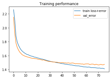
# Show loss curves
# this is both on training and validation data, hence two curves. They track well.
plt.figure()
plt.title('Training performance')
plt.plot(history.epoch, history.history['loss'], label='train loss+error')
plt.plot(history.epoch, history.history['val_loss'], label='val_error')
plt.legend()
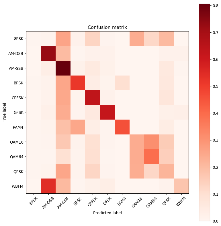
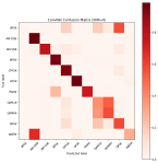
def plot_confusion_matrix(cm, title='Confusion matrix', cmap=plt.cm.Reds, labels=[]):
    #plt.cm.Reds - color shades to use, Reds, Blues, etc.
    # made the image bigger- 800x800
    my_dpi=96
    plt.figure(figsize=(800/my_dpi, 800/my_dpi), dpi=my_dpi)
    #key call- data, how to interpolate thefp vakues, color map
    plt.imshow(cm, interpolation='nearest', cmap=cmap)
    plt.title(title)
    #adds a color legend to right hand side. Shows values for different shadings of blue.
    plt.colorbar()
    # create tickmarks with count = number of labels
    tick_marks = np.arange(len(labels))
    plt.xticks(tick_marks, labels, rotation=45)
    plt.yticks(tick_marks, labels)
    plt.tight_layout()
    plt.ylabel('True label')
    plt.xlabel('Predicted label')
# Plot confusion matrix

#pass in X_test value and it predicts test_Y_hat
test_Y_hat = model.predict(X_test, batch_size=batch_size)
#fill matrices with zeros
conf = np.zeros([len(classes),len(classes)])
#normalize confusion matrix
confnorm = np.zeros([len(classes),len(classes)])

#this puts all the data into an 11 x 11 matrix for plotting.
for i in range(0,X_test.shape[0]):
    # j is first value in list
    j = list(Y_test[i,:]).index(1)
    #np.argmax gives the index of the max value in the array, assuming flattened into single vector
    k = int(np.argmax(test_Y_hat[i,:]))
    #why add 1 to each value??
    conf[j,k] = conf[j,k] + 1

#takes the data to plot and normalizes it
for i in range(0,len(classes)):
    confnorm[i,:] = conf[i,:] / np.sum(conf[i,:])
print (confnorm)
print (classes)
plot_confusion_matrix(confnorm, labels=classes)
[[5.44069641e-03 1.18706103e-02 2.58383619e-01 1.65199327e-02
  1.30873479e-01 8.80403601e-03 3.95687012e-04 2.39093877e-01
  1.22662974e-01 2.04174498e-01 1.78059155e-03]
 [5.07150827e-04 7.25428542e-01 2.00223146e-01 4.86864794e-03
  1.66345471e-02 1.67359773e-02 5.07150827e-04 0.00000000e+00
  0.00000000e+00 1.80545694e-02 1.70402678e-02]
 [1.00310964e-03 3.39051058e-02 8.06801083e-01 2.02628147e-02
  5.22620122e-02 2.18677901e-02 1.00310964e-04 0.00000000e+00
  0.00000000e+00 5.94844016e-02 4.31337145e-03]
 [3.50210126e-03 1.30078047e-02 2.53552131e-01 5.14508705e-01
  3.72223334e-02 1.06063638e-02 1.00260156e-01 2.80168101e-03
  2.50150090e-03 6.08365019e-02 1.20072043e-03]
 [1.50481541e-03 1.39446228e-02 2.46187801e-01 1.18378812e-02
  6.34430177e-01 1.74558587e-02 1.00321027e-04 1.00321027e-03
  0.00000000e+00 7.06260032e-02 2.90930979e-03]
 [6.00841178e-04 2.34328059e-02 2.38133387e-01 7.61065492e-03
  5.56779491e-02 6.22070899e-01 2.00280393e-04 0.00000000e+00
  0.00000000e+00 2.51351893e-02 2.71379932e-02]
 [6.00480384e-03 1.14091273e-02 1.88650921e-01 2.49699760e-01
  3.34267414e-02 8.20656525e-03 4.57065653e-01 1.20096077e-03
  2.50200160e-03 4.01321057e-02 1.70136109e-03]
 [5.38438528e-03 6.78033702e-03 1.64124040e-01 1.41589391e-02
  9.64203809e-02 7.67773457e-03 7.97686709e-04 2.37212085e-01
  3.11995214e-01 1.54551800e-01 8.97397547e-04]
 [4.80384307e-03 4.50360288e-03 9.49759808e-02 1.16092874e-02
  1.00080064e-01 6.20496397e-03 8.00640512e-04 2.38891113e-01
  3.90912730e-01 1.46216974e-01 1.00080064e-03]
 [4.48743518e-03 1.21659354e-02 2.54886318e-01 1.24650977e-02
  1.26844834e-01 9.07459114e-03 2.99162345e-04 2.35839649e-01
  1.25149581e-01 2.17092142e-01 1.69525329e-03]
 [7.94123486e-04 5.44669446e-01 2.02997816e-01 5.95592615e-03
  2.19376613e-02 3.39487790e-02 2.97796307e-04 0.00000000e+00
  0.00000000e+00 1.55846734e-02 1.73813778e-01]]
['8PSK', 'AM-DSB', 'AM-SSB', 'BPSK', 'CPFSK', 'GFSK', 'PAM4', 'QAM16', 'QAM64', 'QPSK', 'WBFM']
# Plot confusion matrix
acc = {}

#this create a new confusion matrix for each SNR
for snr in snrs:

    # extract classes @ SNR
    #changed map to list as part of upgrade from python2
    test_SNRs = list(map(lambda x: lbl[x][1], test_idx))
    test_X_i = X_test[np.where(np.array(test_SNRs)==snr)]
    test_Y_i = Y_test[np.where(np.array(test_SNRs)==snr)]

    # estimate classes
    test_Y_i_hat = model.predict(test_X_i)

    #create 11x11 matrix full of zeroes
    conf = np.zeros([len(classes),len(classes)])
    confnorm = np.zeros([len(classes),len(classes)])
    for i in range(0,test_X_i.shape[0]):
        j = list(test_Y_i[i,:]).index(1)
        k = int(np.argmax(test_Y_i_hat[i,:]))
        conf[j,k] = conf[j,k] + 1

    #normalize 0 .. 1
    for i in range(0,len(classes)):
        confnorm[i,:] = conf[i,:] / np.sum(conf[i,:])
    plt.figure()
    plot_confusion_matrix(confnorm, labels=classes, title="ConvNet Confusion Matrix (SNR=%d)"%(snr))

    cor = np.sum(np.diag(conf))
    ncor = np.sum(conf) - cor
    acc[snr] = 1.0*cor/(cor+ncor)


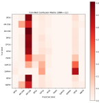


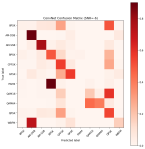
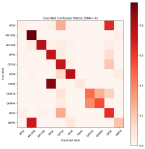


# Save results to a pickle file for plotting later
print (acc)
fd = open('results_cnn2_d0.5.dat','wb')
cPickle.dump( ("CNN2", 0.5, acc) , fd )
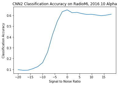
{-20: 0.09679780420860018, -18: 0.09100817438692098, -16: 0.0920767004341534, -14: 0.10591844099603032, -12: 0.12488605287146765, -10: 0.16189799182512885, -8: 0.2592320411537755, -6: 0.4184384164222874, -4: 0.5462107208872459, -2: 0.6337082728592163, 0: 0.650912408759124, 2: 0.6246819338422391, 4: 0.6277533039647577, 6: 0.6162454873646209, 8: 0.6082957619477006, 10: 0.6096539162112933, 12: 0.6031142495020823, 14: 0.596973611367411, 16: 0.6025339366515837, 18: 0.6104410441044105}
# Plot accuracy curve
# map function produces generator in python3 which does not work with plt. Need a list.
# list(map(chr,[66,53,0,94]))
plt.plot(snrs, list(map(lambda x: acc[x], snrs)))
plt.xlabel("Signal to Noise Ratio")
plt.ylabel("Classification Accuracy")
plt.title("CNN2 Classification Accuracy on RadioML 2016.10 Alpha")
Text(0.5, 1.0, 'CNN2 Classification Accuracy on RadioML 2016.10 Alpha')